Spectral Geometry Notes
My most popular tweet of all time was about the eigenvectors of an egg. This wasn't a serious post but people seemed to like it and many curious minds wanted to know what I was getting at with this eggenvector stuff. It felt like the motivation I need to finish compiling my notes on one of my favorite subjects, spectral geometry.
Spectral geometry is a generalization of the Fourier analysis of signals (the 'spectral' part) from the Euclidean domain to curved domains (the 'geometry' part). The major result of spectral geometry is that the eigenvectors of differential operators, primarily the Laplacian, provide a Fourier-like set of orthogonal basis vectors for functions on manifolds.
These notes are about discrete spectral geometry and the applications of spectral methods to discrete geometric data problems found in computer vision and computer graphics.
Some reasons you might be interested:
-
If you are processing three-dimensional geometric data then Laplacian spectral techniques are a must-have tool, they are at the heart of many successful geometry processing algorithms:
- Shape analysis: shape embedding, shape descriptors, shape correspondence.
- Mesh operations: smoothing, parameterization, compression.
- Solving PDEs on geometrical domains.
-
The mathematics involved (functional analysis, differential geometry, spectral theory etc.) have broad applicability beyond three-dimensional geometry, in fields like machine learning & scientific computing.
The Laplacian is one of the most important operators in mathematical physics, used to describe phenomena as diverse as heat diffusion, quantum mechanics, and wave propagation. As we will see in the following, the Laplacian plays a center role in signal processing and learning on non-Euclidean domains, as its eigenfunctions generalize the classical Fourier bases, allowing to perform spectral analysis on manifolds and graphs - Geometric Deep Learning
My goal with this post is that folks come away understanding how to place geometrical data into a Fourier basis and why they would want to do that. You may want to skip around.
Function Spaces
It will be helpful to review a few concepts related to discretization and transformation of one-dimensional functions .
Functions are Vectors
It's important to grok that functions are elements of an infinite dimensional vector space, called a function space. Like all vectors, functions have point-wise addition, scalar multiplication and they can be mapped with linear transformations.
This linear algebraic view of functions is very useful in signal processing where we are generally working with samples of functions, e.g. the discrete pixels in an image. An infinite dimensional function sampled at points is an dimensional vector.
It's useful to summon your intuition around three-dimensional vector-arrows when thinking about function spaces, your functions are now arrows into high-dimensional function spaces.
A simple physical application of function spaces can be found when two lights are superimposed on top of each other, the resulting spectra is the vector addition of the two original spectra.
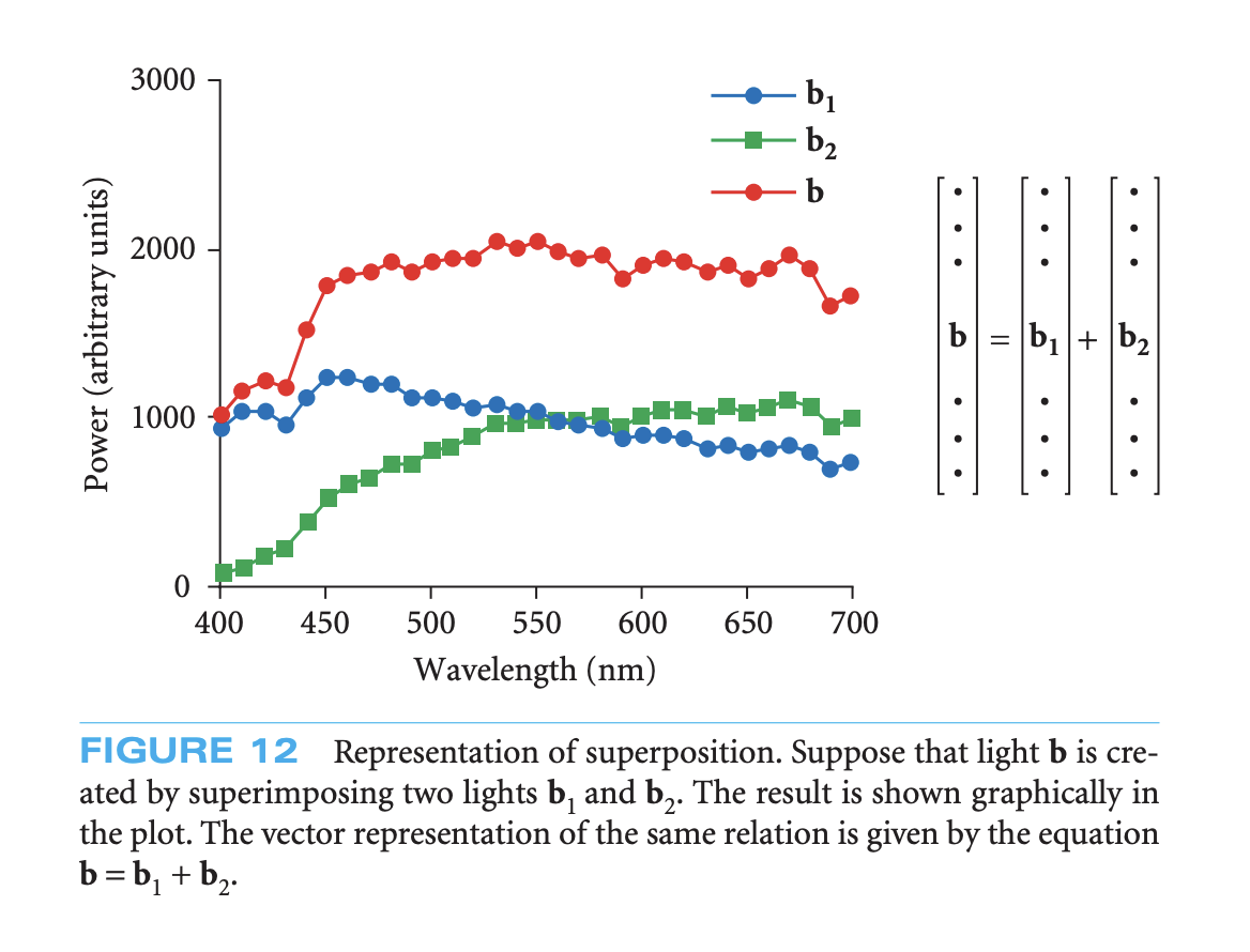
Function spaces can be meaningfully equipped with an inner product, which allows you to project functions into new basis vectors.
An L2 inner product for functions, equivalent to the vector dot product in the discrete case.
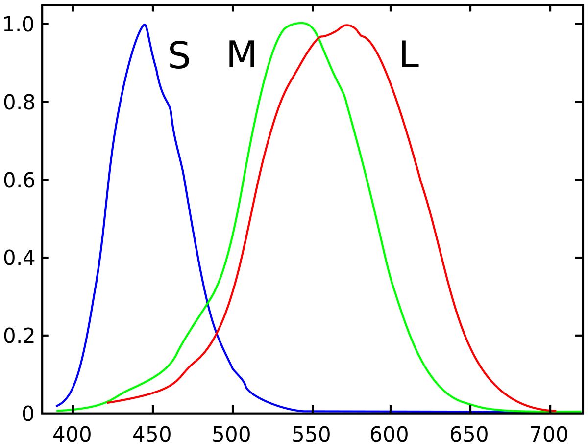
When light hits your eye the resulting color ('tristimulus') can be modeled as the inner product of the light-spectrum-vector projected into the three basis vectors formed by the sensitivity functions of your long, medium and short retinal cones. Color at first order is a dimensionality reduction from an infinite-dimensional function space of visible light beams to a discrete three-dimensional color space.
A discrete signal is a column of coefficients which can be written as the scaled sum of the standard basis vectors.
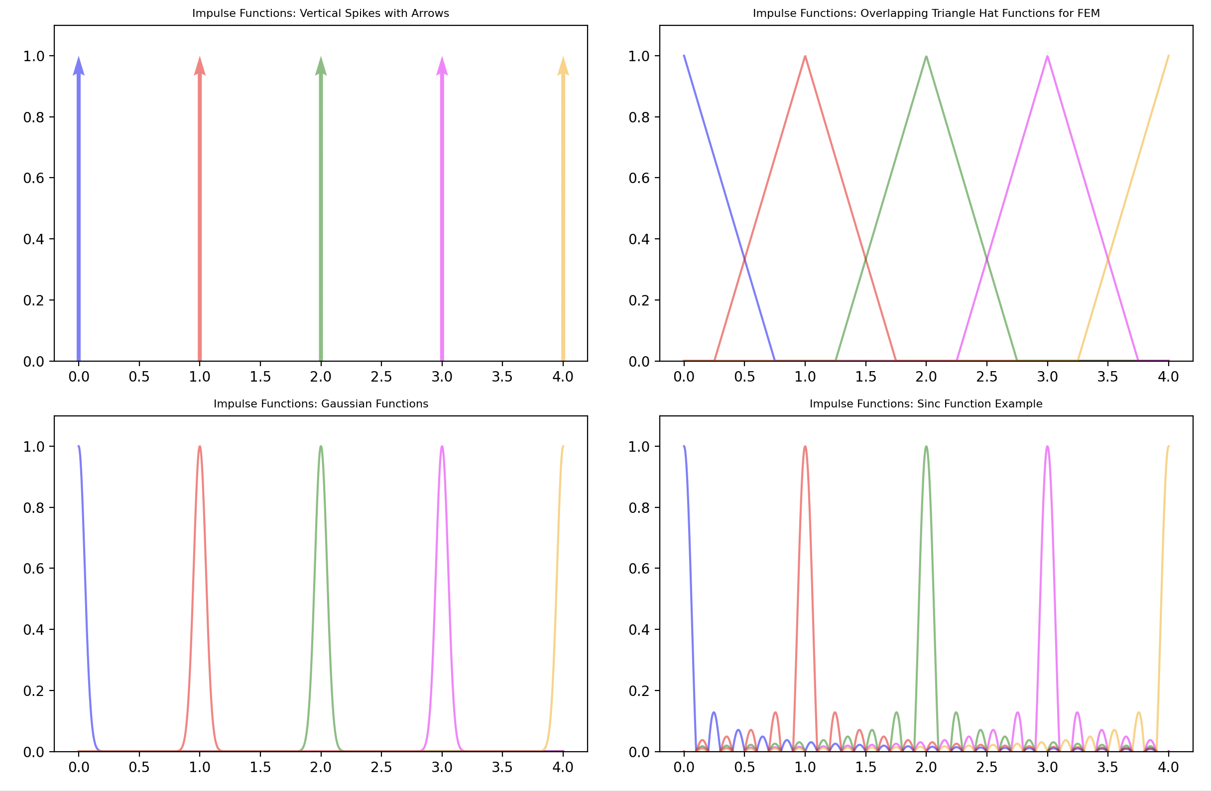
In the functional scenario, we can think of the standard basis functions for our dimensional function space as impulse functions. These are spikes which take on a value of 1 at one location and are zero everywhere else.
Since we often need to work with differentiable impulse basis functions you can approximate them in many ways including triangle 'hat' functions or narrow probability distributions.
Fourier Basis
Since spectral geometry is essentially a generalization of Fourier analysis for manifolds, we need to briefly review Fourier analysis of one-dimensional signals.
The discrete Fourier transform transforms a signal from the standard basis into a set of sin and cos orthogonal basis functions.
Two important differences between the Fourier and standard basis:
- Fourier basis functions are ordered, each basis function has a notion of frequency.
- Fourier basis functions are global, they cover the entire domain whereas standard basis impulse functions only model a local region of the function.
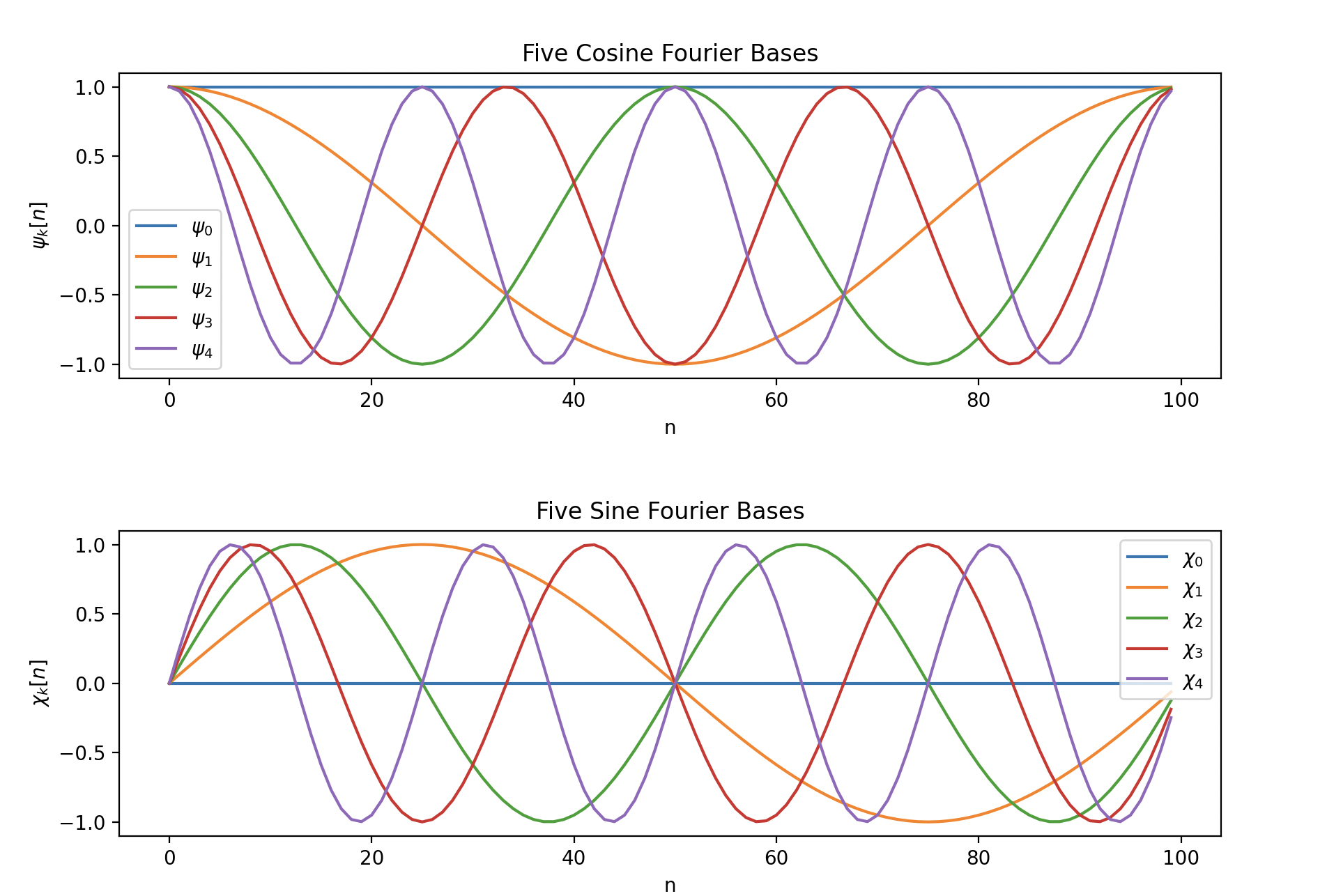
It's easy to overlook, but the Fourier transform projects your signal into two orthogonal bases, one composed of sin functions and one composed of cosine functions.
These are matrices where each row is the frequency basis vector, is the dimensionality of , is the index into the vector.
Correspondingly, after the Fourier transform of your discrete signal you have two new vectors of coefficients and .
These vectors are you new Fourier representation of your signal, each element of the vector is the scale factor for the frequency basis vector, which comes from the projection of your signal into each basis function.
Reconstruction of the signal back in the standard basis:
Note in real-world implementations of the discrete Fourier transform, and are cleverly combined into a single vector of complex numbers , with the real part represented the sin coefficients and the imaginary part representing the cosine coefficients.
Most natural signals are highly structured and can be represented efficiently in the Fourier basis, with far fewer dimensions than the original signal.
Discrete Differentiation
Anytime you have an interesting function you should be pondering its derivative.
If our discrete function is a finite dimensional vector, how do we take the derivative of a vector?
You may or may not remember that differentiation is a linear process. In the discrete setting we can create a finite differences matrix and cast differentiation of one-dimensional functions as a matrix multiplication problem.
This is not the most efficient or numerically stable way to compute finite differences, but it does highlight the idea of a differential operator matrix, which we can study using matrix analysis methods like eigendecomposition. This will be a very useful view when we start talking about discrete differential operators on manifolds.
Let's quickly convince ourselves that computing a derivative of a one-dimensional function can be cast as a matrix multiplication problem.
def central_differences_matrix(n, delta):
    d = np.zeros((n, n))
    for i in range(1, n-1):
        d[i, i-1] = -1
        d[i, i+1] = 1
    d /= (2 * delta)
    return d

# generate sample points
x = np.linspace(0, 10, 100)

f = np.sin(x) # our function
dfdx = np.cos(x) # our function's analytic derivative

# our 1D discrete derivative operator, an nxn matrix
differential = central_differences_matrix(len(x), x[1] - x[0])

# f′ = df ⋅ f
# our function's numerical derivative
# computed with a discrete differential operator
dfdx_approx = differential.dot(f)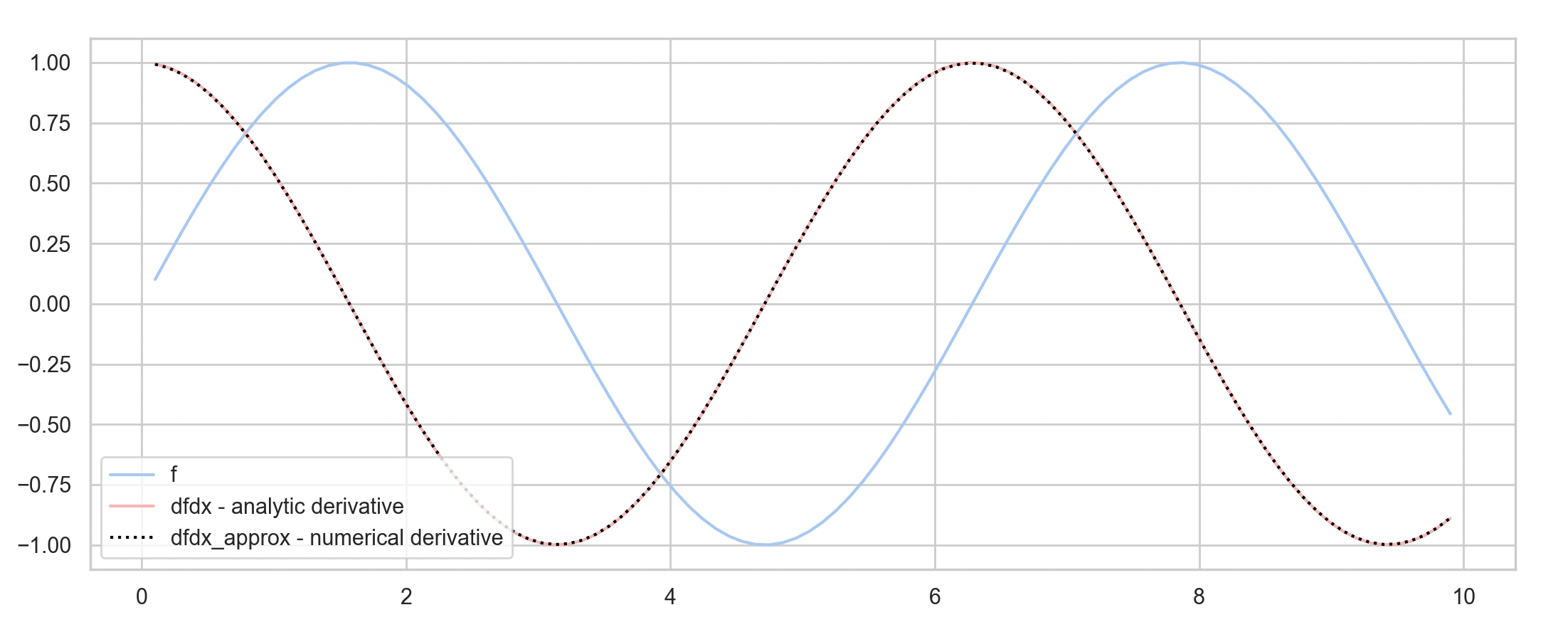
Differential Geometry
Manifolds
Manifolds are a formalism used to model smooth curved shapes, their defining characteristic is that at a certain scale they are locally flat, you can treat local patches of the manifold as if they were the Euclidian plane. Differential geometry is concerned with definitions of curvature on manfiolds and tools for doing calculus with functions defined on manifolds.
"A manifold, generally speaking, is a topological space which resembles Euclidean space locally. A differentiable manifold is a manifold for which this resemblance is sharp enough to allow partial differentiation and consequently all the features of differential calculus on ." - Modern Differential Geometry of Curves and Surfaces, 2006
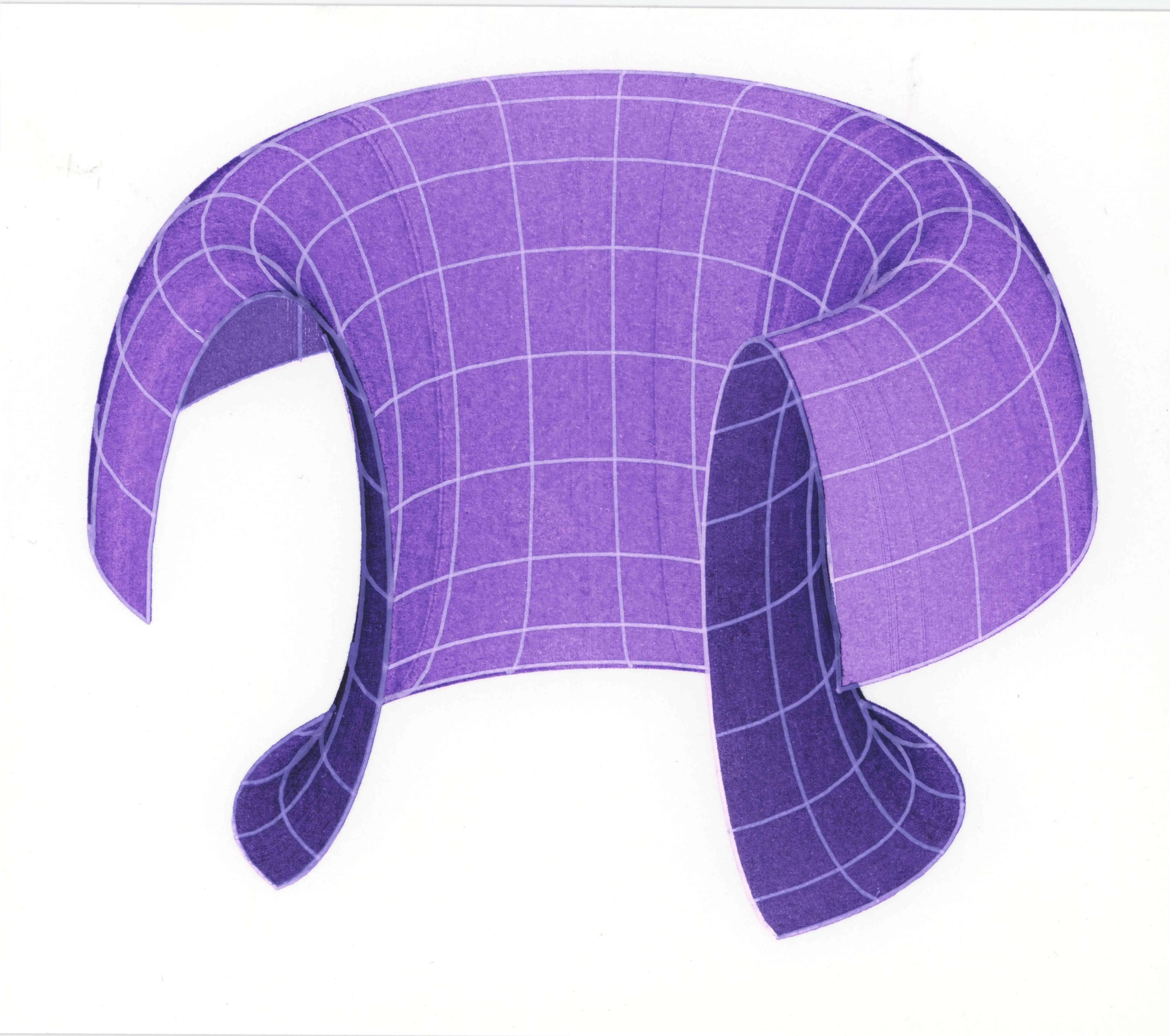
Author's sketch of a partial torus, a smooth analytic manifold.
Many analytic manifolds are given by a parameterization but the theory of manifolds can be fruitfully applied to arbitrary smooth shapes for which there is no simple analytic form. The surfaces of many real world objects can be well approximated as manifolds.
"The subject of 'shape' is too enormously varied to treat even superficially in a text like this...Today's small piece is basically about arbitrary smooth lumps of space such as could be occupied by your typical potato" - Solid Shape, 1991
Manifolds theory provides us with various definitions of curvature and a framework for calculus on curved domains.
Discrete Geometries
Point clouds are an unordered collection of positions – they are commonly produced by range cameras and 3D scanners where they can be interrupted as a noisy sampling of the surface positions of an underlying manifold.
Triangle meshes are collections of triangular faces connected at edges. Whereas point clouds can model surfaces, volumes or even curves – triangle meshes are more constrained to modeling surfaces and have a tighter connection to the concept of a surface manifold.
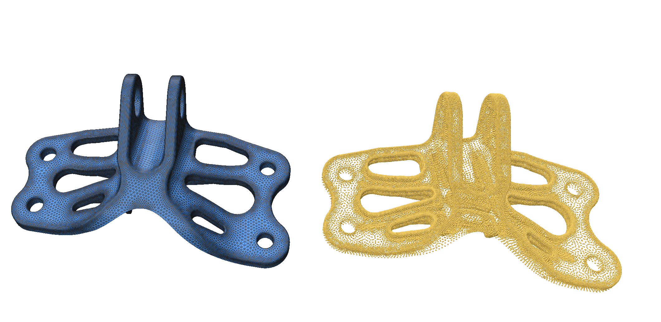
A bracket from the SIMJEB dataset , in triangular mesh (left) and point cloud (right) forms.
A powerful feature of spectral techniques is that they are domain agnostic – spectral techniques can be readily applied to a large number of different discrete geometries (meshes, voxels, point clouds, even graphs) provided there are discrete linear operators defined on those geometries. Discrete linear operators are the link between our discrete geometric data and the continuous spectral theory of manifolds.
Discrete differential geometry is a hot topic and I cannot recommend Keenan Crane's notes. on the subject enough.
Intrinsic Geometry
An important concept in differential geometry is that of intrinsic vs extrinsic shape properties. Extrinsic geometry is concerned with the way a shape is embedded into Euclidian space. The size/scale/position/pose/rotation of your object all depend on the extrinsic frame of reference.
Intrinsic geometry is invariant to the embedding and only has to do with the curvature of the shape.
Human perception is equipped with an intuitive notion of intrinsic geometry, you would probably say two cups that were rotated differently were the same 'shape'.
On the other hand, it's slightly less obvious that the bending of a sheet of paper in one direction is, like rotation, entirely an extrinsic transformation.
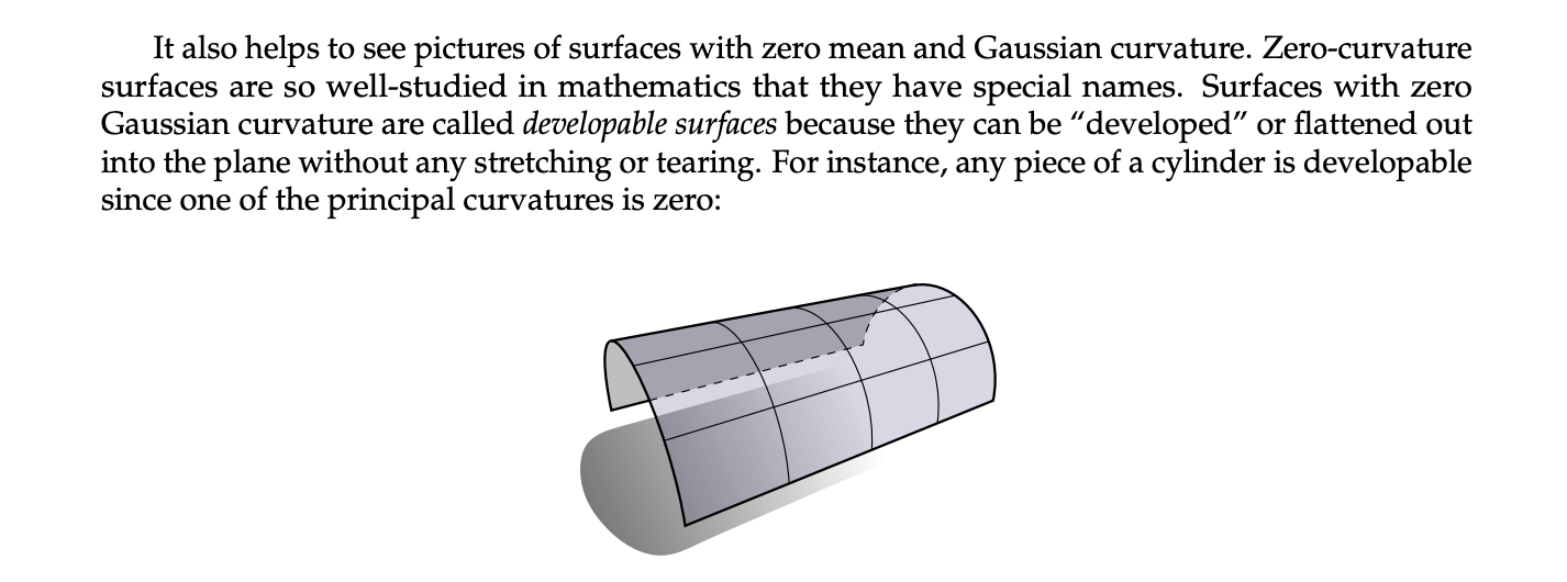
A bent sheet of paper, credit: Keenan Crane
You can bend a sheet of paper in one direction or the other but not both because bending in two directions would change the Gaussian curvature of the surface, an intrinsic property. For materials like paper, which is inflexible to changes in area, this would cause a tear or crinkle.
Triangle meshes have both intrinsic and extrinsic properties, each vertex of the mesh contains a tuple of coordinates that define a shape's position in space, which is the extrinsic concern. The angles and lengths of edges at each vertex encode the intrinsic properties of the shape.
These notes will discuss how to use spectral geometry to shed the notion of vertex coordinates and analyze a discrete shape entirely from an intrinsic point of view.
About Graphs
Graphs, which consist of nodes and edges, have their own spectral theory which predates spectral methods for discrete geometry.
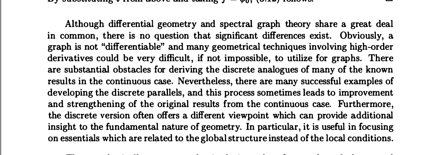
Fan Chung, Spectral Graph Theory, 1992
I find it fascinating that graphs are an inherently discrete domain, while triangle meshes are a graph which is a discrete approximation of an inherently smooth domain.
Some graphs resemble manifolds (like the edges of triangular meshes); the more a graph deviates from a smooth manifold the more spectral geometry assumptions breakdown. For example there's no concept of tangent spaces on graphs.
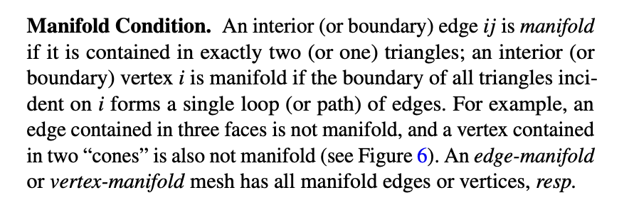
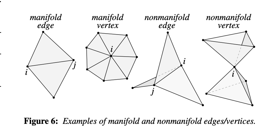
A Laplacian for Nonmanifold Triangle Meshes, 2020
A major unifying concept between geometry and graphs is the Graph Laplacian, a discrete laplacian operator that that only takes into account connectivity and not edge lengths or angles, which allows it to be directly applied to both mesh geometry and graphs.
Like geometric deep learning for manifolds, graph neural nets for processing graph based domains have become an important research area in machine learning.
Signals on Surfaces
The most familiar time and space varying signals, like images, radio, sound etc, are functions on the Euclidean domain.
Now it's time to discuss functions on manifolds.
Scalar and Vector Fields
By function on a manifold, I mean a function that assign a real number to each point on a manifold . .
An example would be the function that returns the temperature at each point on a surface.
Discrete scalar fields are represented by a single list of numbers which is mapped onto the mesh by being in the same order as the list of vertices in the mesh data-structure, f[i] corresponds to vertices[i].
In the context of manifolds such functions are often called scalar fields and functions that assign a vector to each point on the manifold are vector fields. Our temperature function is a scalar field and the gradient of our temperature function is a vector field.
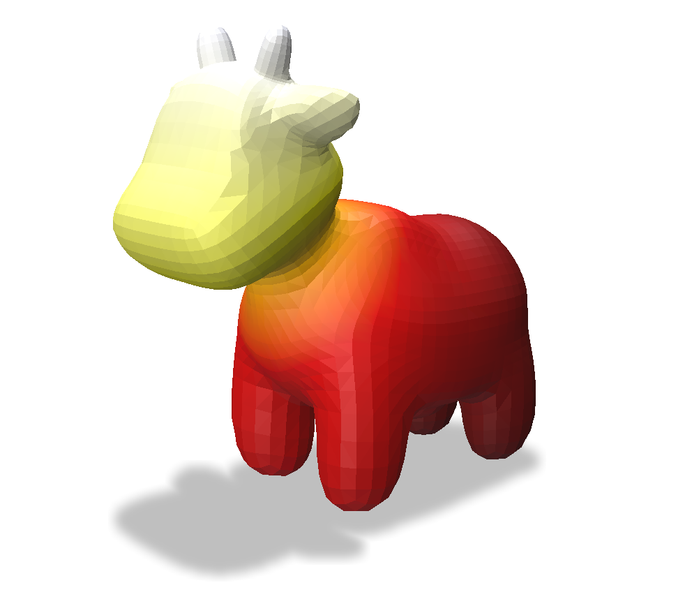
Heat map visualization of a function defined on the vertices of a triangle mesh.
In a vector space all vectors are attached to the origin, but in our vector field each vector is attached to a different point on the mesh – this is accomplished by assigning each point on the manifold it's own vector space called a tangent space .
If you would like to compare two vectors in a vector field you first need to transport one into the other's tangent space by sliding it along the manifold. This is a major area of study in differential geometry known as parallel transport .
This is a good example of the extra machinery required to deal with functions on manifolds, in Euclidean space you could directly compare two vectors from a vector field as if they were in the same vector space.
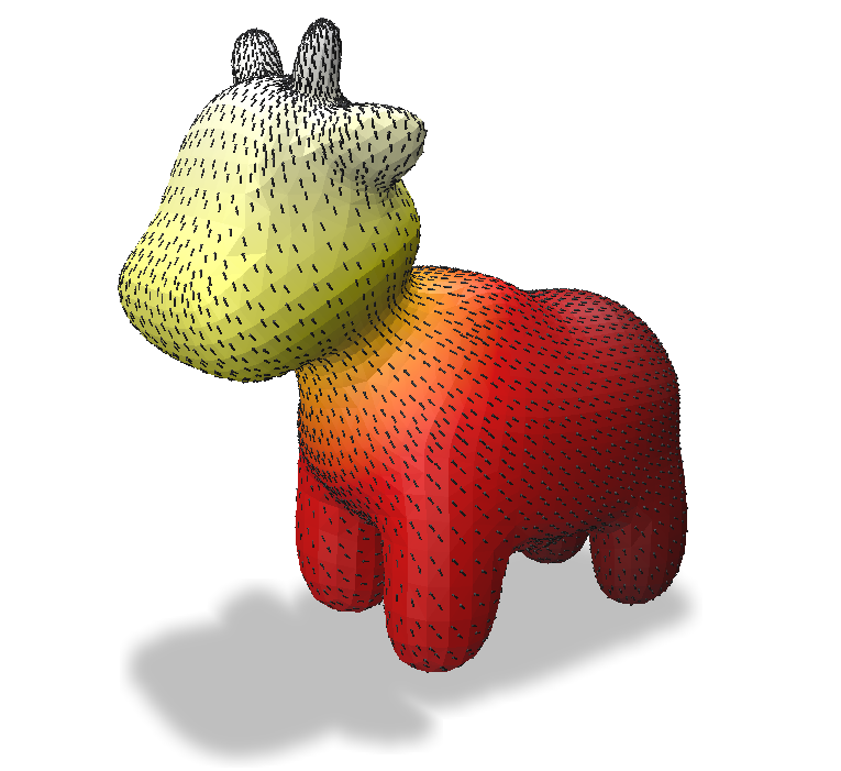
Arrow visualization of a vector field attached to the faces of a mesh.
Differential Operators
Compared to our one-dimensional Euclidean examples linear operators on manifolds are a bit more exciting. We have access to the standard operations of multi-variable calculus, notably gradients and laplacians – except constructed as operators that apply to functions on curved manifolds. We can do calculus on shapes!
Make note of the type signatures here, operators are not the same as their outputs. A differential operator is a linear map on function spaces, it maps the function to a new function related to the derivative of . In computer science terms we'd call this a higher-order function, consuming a function and outputting a new function.
-
- A function which associates each point on with a scalar.
-
gradient:
- A function that associates each point on with a vector pointing in the direction of greatest change. The vectors actually lie flat against the manifold in the tangent space . Each point on a manifold has its own tangent space.
-
gradient operator:
- Maps the space of scalar-valued functions on manifolds to the space of vector-valued functions on manifolds
If you're like me, an example would help right about now. Let's work computing the gradient of a function on a mesh in Python. We'll use the IGL library to construct the mesh gradient operator (a matrix) and the Polyscope library to visualize it.
Note this example uses the x position of all vertices as the example function, we should expect that its gradient flows along the mesh in the most x direction possible.
import numpy as np
import polyscope as ps
import igl

def normalize_vector(V):
    return V / np.linalg.norm(V)

# load a triangle mesh, V is a list vertices F is a list of Faces
V, F = igl.read_triangle_mesh(spot)

# f is a per-vertex scalar field (it's just the x coordinates of the mesh in this example)
f = V[:,0]

# discrete gradient operator, a matrix that maps per-vertex values to per-face vectors
grad = igl.grad(V, F)

# gradient of f is a vector field defined on the center of each face
∇f = normalize(grad.dot(f).reshape(F.shape, order="F"))

# visualize
ps.init()
mesh = ps.register_surface_mesh("mesh", V, F)
mesh.add_scalar_quantity("f", f, cmap="viridis", enabled=True)
mesh.add_vector_quantity("grad_f", values=∇f, defined_on="faces", enabled=True)
ps.show()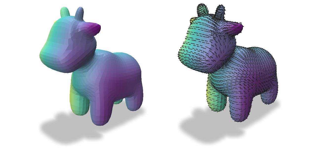
The x coordinate function and its gradient.
The Laplacian
Finally, it's time to introduce the Laplacian operator for functions on manifolds. The Laplacian computes the difference between a function at a point and the average value of that function in neighboring points.
-
Laplacian:
- A function which represents the sum of second derivatives of a function
-
Laplacian operator:
- maps scalar-valued functions to their Laplacian, another scalar-valued function
A common definition of the Laplacian is that it is the divergence of the gradient.
Given a triangle mesh with N vertices, an NxN Laplacian matrix can be constructed and applied to N dimensional function vectors on the shape.
Because its construction involves edge lengths and angles from the mesh, the matrix captures all intrinsic information about the shape, while shedding all information about the meshes embedded position.
This is huge, don't miss it. The Laplacian operator isn't just an map on function spaces, the operator is actually is a stand-in data structure for analyzing the shape from an intrinsic point of view.
You can be sure that any analysis done on a shape's discrete Laplacian matrix is invariant to scale/pose. It's not hard to imagine the utility of this, if you are trying to match objects at different scales or poses you would definitely want to compare them using intrinsic data structures.
Here are three commonly used algorithms to construct discrete Laplacian matrices:
-
Graph Laplacian: Only considers the connectivity of a triangle mesh and not angles between edges or lengths of edges, works well when mesh connectivity is highly indicative of geometry.
-
Cotan Laplacian: A true geometric Laplacian which considers lengths and angles as well as connectivity, more accurate than the Graph Laplacian but less numerically stable.
-
Robust Laplacian: An spectacular recently introduced Laplacian which works on meshes & point clouds and remains stable in the presence of malformed and noisy data.
An important paper by Wardetzky et al, Discrete Laplace Operators: no free lunch , describes how no single discretization of the Laplacian can capture all natural properties of the smooth Laplacian.
I use the Robust Laplacian for everything now, there is a stand-alone python implementation on pypy. I recommend the paper which won best paper at SGP 2020: A Laplacian for Nonmanifold Triangle Meshes, Sharp et al.
Spectral Methods
Eigendecomposition of the Laplacian
Anytime you have a matrix you should be pondering the meaning of its eigenvectors and eigenvalues.
I've told you already that the eigenvectors of the discrete Laplacian form a set of Fourier basis functions on the shape, but I think this is best appreciated visually.
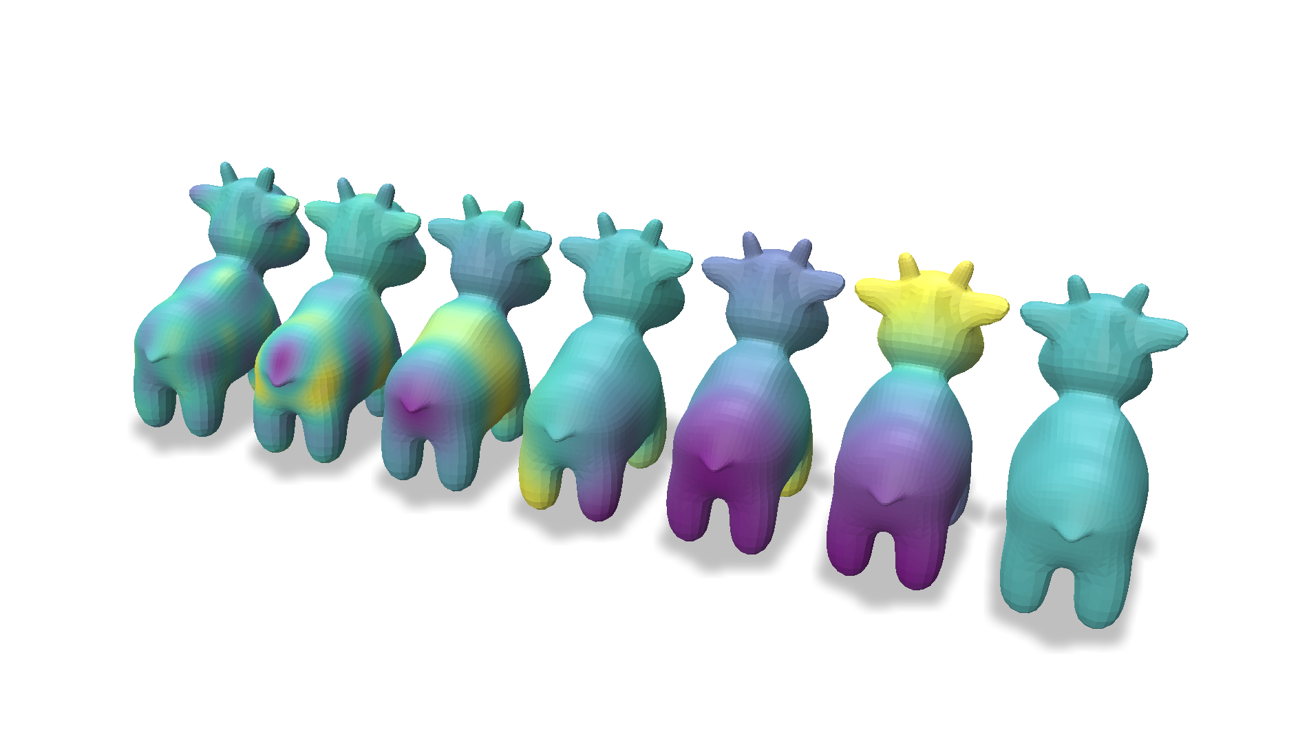
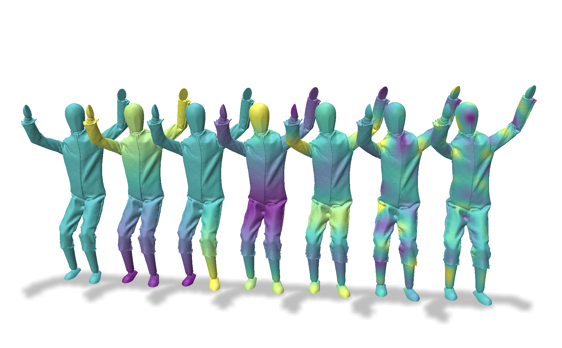
In this example I've computed a discrete Laplacian for a mesh and then visualized its eigenvectors as functions on the mesh.
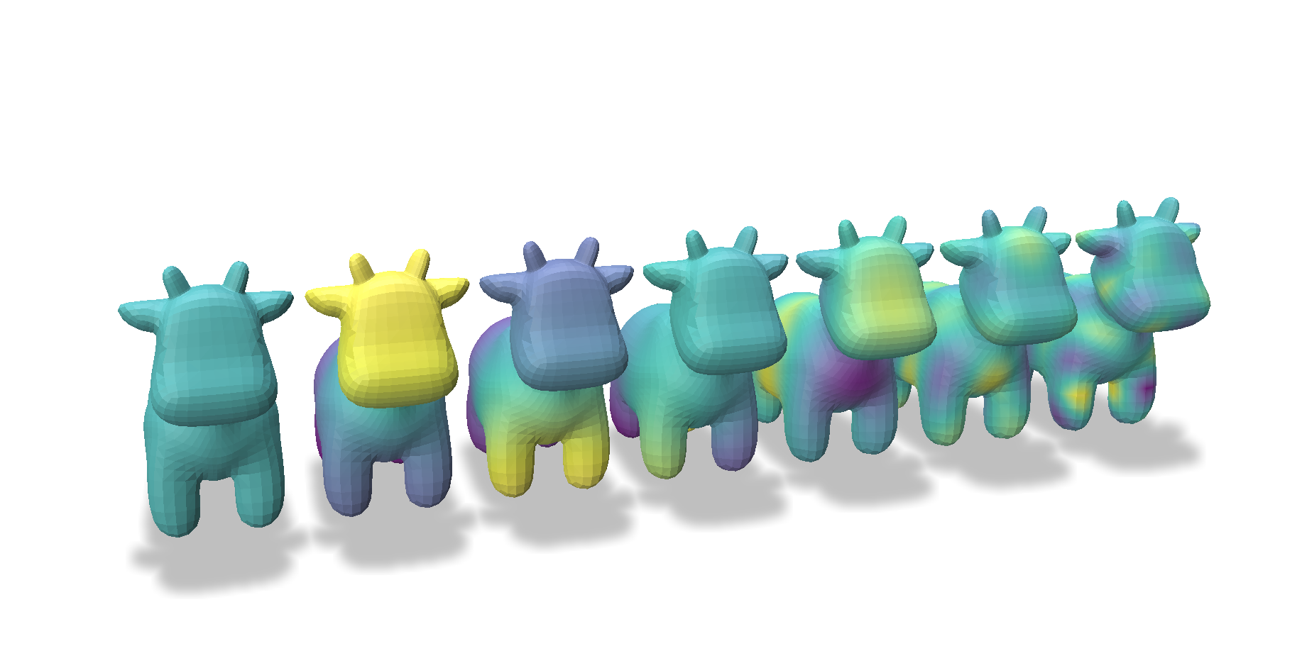
[0,1,2,5,10,50,100] eigenvectors of the shape (left to right).
[0,1,2,5,10,50,100] eigenvectors of the shape (right to left).
code for eigenfunction visualization
The behavior here is surprising, almost magical, the eigenvectors of the Laplacian matrix tend to isolate salient parts of the geometry in an ordered way. The zeroth eigenvector is a constant function but the first eigenvector splits the shape in two along the dominant axis, very interesting.
As the eigenvalues get smaller the oscillation of the function gets smaller and highlights different parts of the geometry.
These functions are a type of Fourier series for functions defined on a mesh; this is the real essence of spectral geometry.
Here's another:
It's important to remember that each shape has its own unique set of unique Fourier bases that depends on the curvature and topology of the shape. This makes them somewhat less useful than the typical Fourier series, where signals all share the same set of Euclidean basis functions.
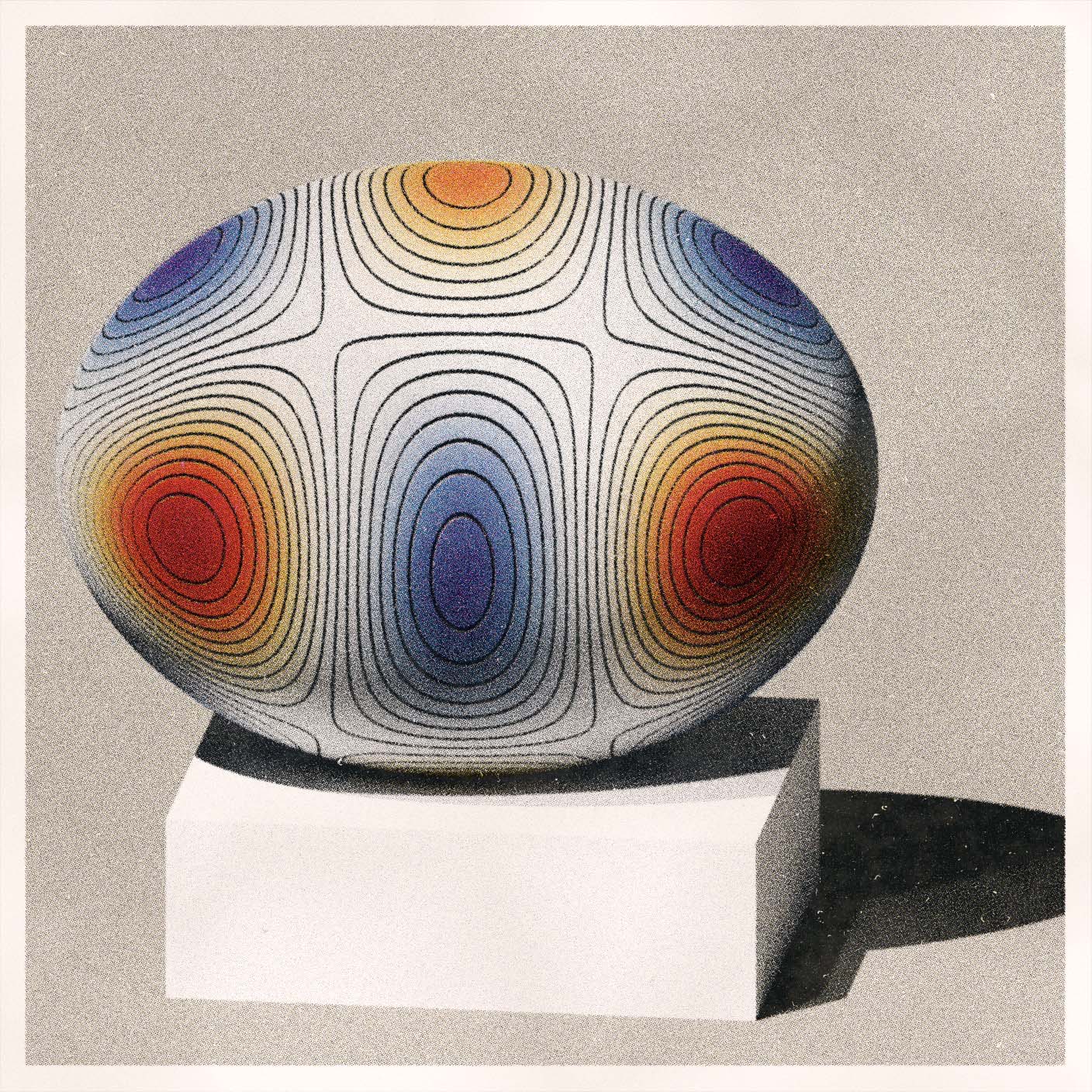
These functions may be familiar to physicists, on the spherical domain they are identical to the spherical harmonic functions, which are solutions to the Laplace equation on the sphere.
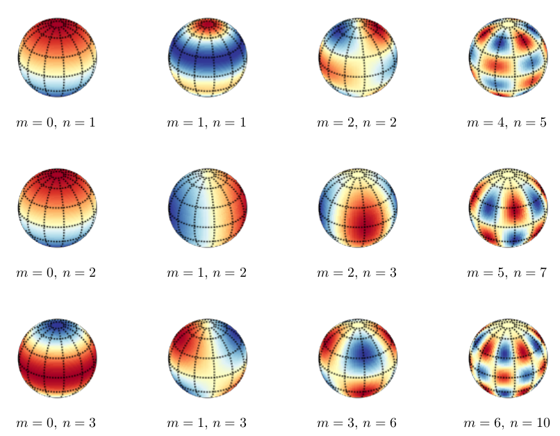
Spherical harmonics, source: stack exchange
Now you understand what the Eggenvector was all about.
Mesh Representation
We now have a set of interesting global basis vectors for functions on our mesh, just like in classical Fourier analysis we can project any other function into each of our basis vectors and store the coefficients as the Fourier representation of our mesh.
Presently functions on our mesh have an dimensional vector representation where is the number of vertices in the mesh, however in the Fourier bases we might be able to get away with representing functions in a small number of Fourier bases and truncating the rest.
In order to visualize how well this works, we will project the mesh coordinate functions into the top k Fourier bases and then convert back into the spatial domain and see how well the mesh shape is preserved.
The routine goes like this:
- Compute the discrete laplacian
- Project vertex coordinates into your spectral basis.
- Truncate spectral basis to be low dimensional.
- Use spectral representation for your application.
- Reconstruct into spatial domain when mesh is needed.
This is all analogous to the signal change of basis / reconstruction in our one-dimensional Fourier section.
code for spectral mesh compression
As we use fewer and fewer eigenvectors the shape loses it's high frequency components and retains only it's low frequency forms, again, magic.
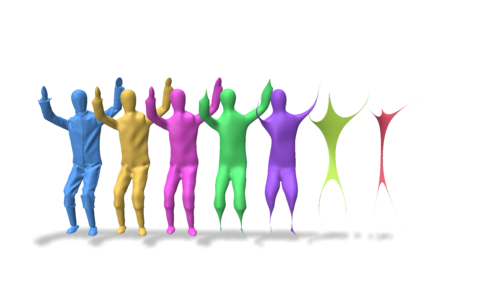
500,300,100,50,10,5 eigenvector representation.
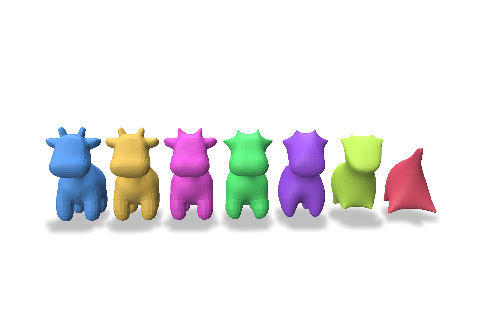
500,300,100,50,10,5 eigenvector representation.
We've created dimensional representations of our shape that can retain a surprising amount of accuracy found in the dimensional original.
Applications
Because spectral methods make use of global basis functions, they struggle to represent fine detail in large datasets. I think this is the reason spectral methods are not as popular as Finite Element Methods for many high dimensional data problems – I am not an expert here though.
Spectral Clustering
Probably the most successful uses of spectral methods in geometry are spectral embedding and spectral clustering,
The values of the first eigenvectors can be considered a dimensional embedding of the entire mesh.
This is what a three-dimensional spectral embedding of the Stanford bunny looks like. To spell it out, each i-th vertex of the original mesh is given a new spatial coordinate equal to the i-th value of each eigenvector, in this case the first three.
K-dimensional spectral embeddings can be efficient spaces to apply clustering algorithms, such as k-means clustering, to data that may be difficult to cluster in the spatial domain due to high-dimensionality.
Clustering performed on the embedding space has the advantage of being extrinsically invariant, you will get the same clusters for the same object shapes in different poses! This the magical intrinsic data analysis that was promised.
Many real world deformable objects deform extrinsically but not intrinsically. Essentially, the joints move but the surface doesn't change area. By analyzing the laplacian we can strip out all extrinsic differences. In the example below the pose of the doll would not change the clustering.
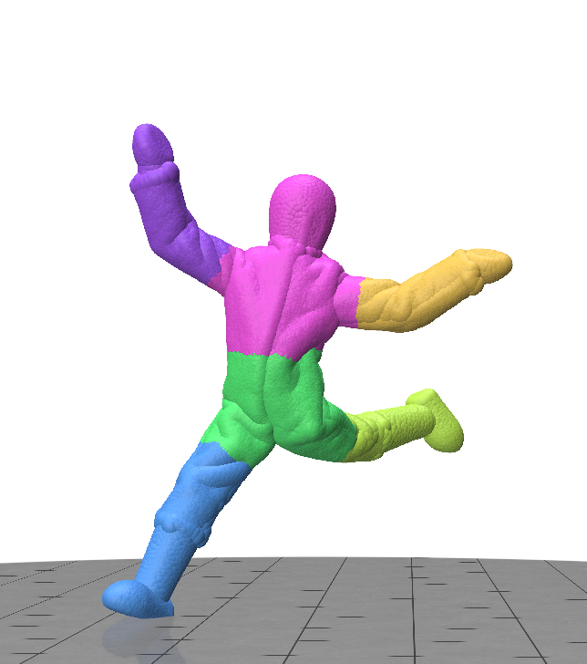
K-means clusters on the spectral embedding of this shape.
It's easy to visualize three dimensions but you can do spectral clustering in high dimensions to capture higher frequency shape features, below we use 100 dimensions for our clustering example.
import numpy as np
import igl
from scipy.cluster.vq import kmeans2
from scipy.sparse import linalg as sla
import robust_laplacian
import polyscope as ps

# Spectrally embed the mesh into a space with
# this many dimensions
spectral_embedding_dimensions = 100

# split objects into this many segments
num_segments = 7

def k_spectral_embedding(verts, faces, k):
  """ Embed vertices into k dimensions """
  L, M = robust_laplacian.mesh_laplacian(verts, faces)
  evals, evecs = sla.eigsh(L, k=k+1, M=M, sigma=1e-8)
  return(evecs / np.sqrt(evals))[:, 1:]

# Load a shape
V,F = igl.read_triangle_mesh("mesh.obj")

# Create the embedding
embedded_points = k_spectral_embedding(V,F, k=spectral_embedding_dimensions)

# Do k-means clustering on the embedding
_, per_point_labels = kmeans2(embedded_points, num_segments, minit='points')

# Visualize the clusters
ps.init()
for i in range(0, num_segments):
  ps.register_point_cloud(
    f'cluster_{i}', V[per_point_labels==i], radius=0.05)
ps.show()
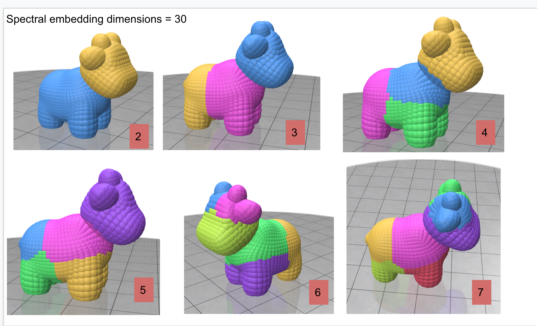
Differing numbers of k-means clusters on the spectral embedding.
A detailed review of spectral segmentation can be found in Discrete Laplace-Beltrami operators for shape analysis and segmentation
Functional Maps
A popular paper, Functional Maps: A Flexible Representation of Maps Between Shapes , proposed mapping functions between shapes by placing the functions into their spectral bases and then solving for a linear transformation (the 'fmap') which maps between two shapes respective spectral bases.
This has potential as a method for transforming one deformable shape into another.
While elegant this approach has so far struggled to find success in real-world applications, I suspect that functional maps may yet have its moment in signal processing on manifolds.
This paper is largely what motivated these notes.
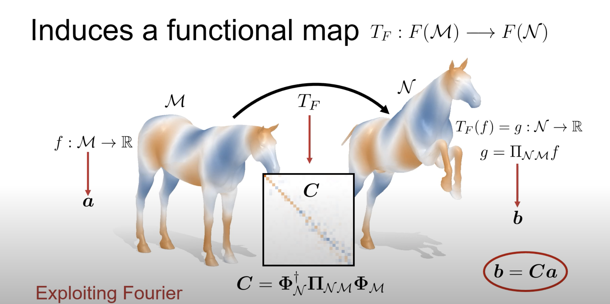
Diagram from the Functional Maps paper
Compression
The scheme above, where we truncate high frequency eigenvectors to simplify the shape, has been proposed as as mesh compression technique. It's interesting that it hasn't taken it off, to my knowledge no major formats use lossy geometry compression.
One issue here is that unlike with JPEG compression, each shape has its own spectral basis. This means you cannot easily decode a shape from its spectral coefficients without passing along the basis functions as well.
Resources
Some materials that went into these notes and which I recommend.
Fourier Analysis
[chapter] Data-Driven Science and Engineering (chapter 2) , 2019
[notes] Generalizations of Fourier analysis
Spectral Theory
[book] Spectral Graph Theory, 1997
[chapter] Numerical Geometry of Non-Rigid Shapes (chapter 8), 2008
[survey paper] Spectral Mesh Processing, 2009
[paper] Functional Maps: A Flexible Representation of Maps Between Shapes, 2012
[book] Spectral Geometry of Shapes, 2019
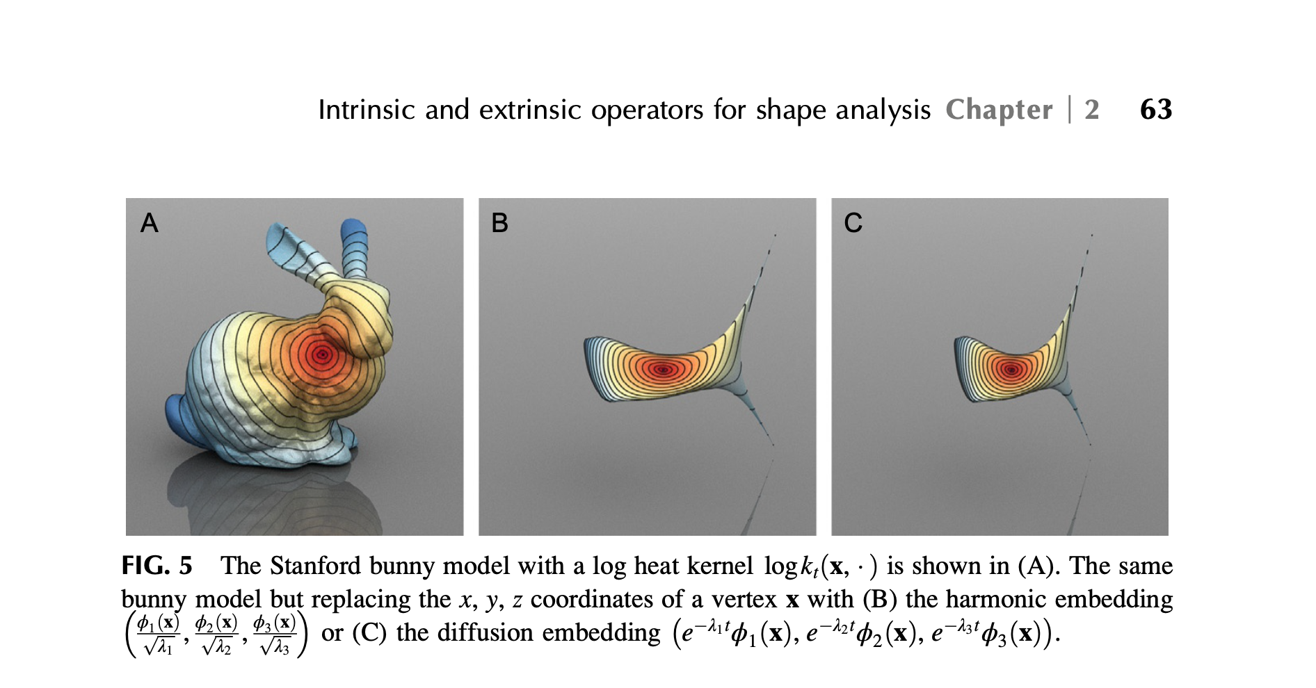
[chapter] Intrinsic and extrinsic operators for shape analysis, 2020
Discrete Differential Geometry
[paper] Discrete Laplace Operators: no free lunch, 2007
[paper] A Laplacian for Non-manifold Triangle Meshes, 2020
[notes] Discrete Differential Geometry: An Applied Introduction
Differential Geometry
[book] The Shapes of Things, 2015
[book] Solid Shape, 1991
Machine Learning
[paper] Geometric Deep Learning , 2021